Excel Marksheet: How to Create a Marksheet in Excel
(8 Simple Steps)
Creating an Excel mark sheet is one of the most common requirements for teachers, coaching centers, schools, and Excel learners. Whether you’re preparing student results or learning Excel formulas, building a mark sheet Excel template is an excellent way to improve your skills.
In this beginner-friendly guide, you will learn how to make a marksheet in Excel, how to enter data, apply formulas, calculate total, percent, result, and grade—along with formatting tips and expert shortcuts.
Table of Contents
What Is an Excel Mark Sheet?
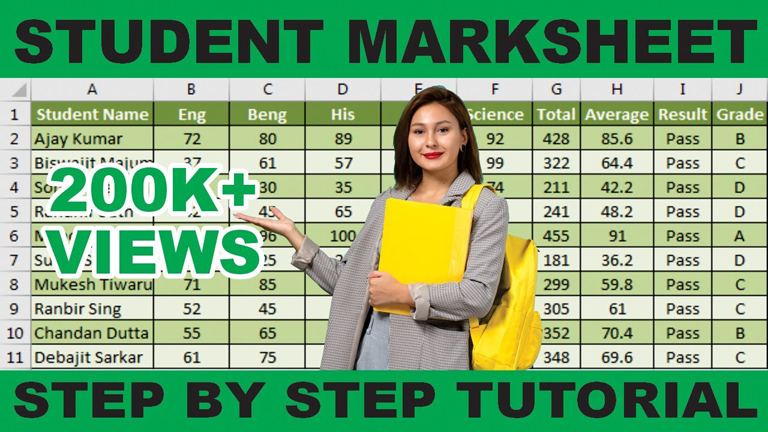
An Excel mark sheet is a worksheet in Microsoft Excel where you record student marks, calculate totals, averages, results, and grades. Teachers and institutions use it because Excel automatically performs calculations using formulas.
This tutorial covers:
Student data entry
Subject marks
Total marks
Average/percentage
Pass/Fail result
Grades (A, B, C, D, Fail)
Table formatting
Why Learn to Create a Marksheet in Excel?
Before jumping into the tutorial, let’s understand why Excel is the best tool for creating marksheets:
1. Saves Time: Once formulas are set, Excel automatically calculates results for all students.
2. 100% Accuracy: No human calculation errors—Excel does all computations perfectly.
3. Reusable Template: You can use the same grade sheet every month, term, or year.
4. Easy to Format: Excel allows color coding, borders, conditional formatting, charts, and more.
5. Professional Presentation
6. Well-designed marksheets look clean and trustworthy.
Step By Step Tutorial
Step 1: Set Up the Marksheet Layout
Open a new Excel sheet.
In the first row, enter the main headers that will structure your marksheet.
A simple and effective header structure is:

| A | B | C | D | E | F | G | H | I | J |
|---|---|---|---|---|---|---|---|---|---|
| Name | Eng | Ben | His | Geo | Science | Total | Average | Result | Grade |
You can customize subjects as per your school or class.
Tips for Better Header Design
Make headers bold
Increase row height
Use colors for better readability
Apply borderlines to the header row
Step 2: Enter Student Details and Marks
Start entering the following:
Student names
Marks for each subject
Example:
| Name | Eng | Ben | His | Geo | Science |
|---|---|---|---|---|---|
| Amit | 78 | 66 | 72 | 80 | 75 |
| Riya | 55 | 49 | 60 | 52 | 58 |
| Soham | 90 | 88 | 85 | 91 | 89 |
Once data is entered, you are ready to apply formulas that will make the marksheet dynamic.
Step 3: Calculate Total Marks Using Excel Formula
To automatically calculate a student’s total marks:
Click on G2
Enter the formula:
=SUM(B2:F2)Press Enter
You will see the total marks for that student.
Now copy the formula down to apply it to other students.
Why This Works
SUM(B2:F2) adds all subject marks for one student at a time.
Step 4: Calculate Average or Percentage
To calculate the average:
Click on H2
Enter the formula:
=AVERAGE(B2:F2)Press Enter
This displays the average marks for the student.
Copy this formula down to calculate averages for all students.
Percentage vs Average
If each subject has the same maximum marks, then:
Average = Percentage
If subjects have different weightage, then a different formula is required.
Step 5: Determine Pass or Fail Status
In this tutorial, the rule is:
If the Average ≥ 35, the student is Pass
Otherwise Fail
To apply this rule:
Click on I2
Enter the formula:
=IF(H2>=35,"Pass","Fail")Press Enter
Copy the formula down for other students.
✔ Tip:You can change the passing criteria (e.g., 40 or 50) as you wish.
Step 6: Assign Grades Automatically
Now we create a grading system based on the student’s average.
Grading Criteria
A → 90 and above
B → 70 and above
C → 50 and above
D → 35 and above
Fail → below 35
Formula to Calculate Grade
Click on J2 and enter:
=IF(H2>=90,"A",
IF(H2>=70,"B",
IF(H2>=50,"C",
IF(H2>=35,"D","Fail"))))
Hit Enter.
Copy the formula down to apply grading for all students.
✔ Why We Use Nested IF
A nested IF allows Excel to check multiple conditions step-by-step.
Step 7: Format the Marksheet Professionally
A good-looking marksheet is easier to read and understand.
Basic formatting ideas:
Make headers bold and larger
Use light background color on headers
Apply borders around the entire table
Align text centrally
Use conditional formatting for:
Fail = red color
Pass = green color
Add Conditional Formatting (Optional)
To highlight FAIL students:
Select the Result column
Go to Home → Conditional Formatting → Highlight Cell Rules
Choose Text contains “Fail”
Select red fill
This gives an instant visual cue.
Step 8: Convert Your Marksheet Into a Printable Format
To prepare your grade sheet for printing:
Set page border
Adjust column width
Freeze top row
Add school logo or header
Insert page numbers
This makes the final output clean and professional.
Pro Tips
Here are some extra suggestions to make your marksheet more powerful:
1. Add Maximum Marks Column
Helps calculate exact percentages.
2. Add Rank Calculation
Use:
=RANK(G2,$G$2:$G$50,0)
3. Add Remarks Section
Example:
-
Excellent
-
Good
-
Needs improvement
4. Use Data Validation
Restrict subject marks to valid ranges.
5. Protect Sheet
Lock formulas so they cannot be modified accidentally.
FAQs
1. How to make marksheet in Excel quickly?
Follow this tutorial: enter headings → insert marks → use SUM & AVERAGE → apply result & grade formulas.
2. Excel me marksheet kaise banaye?
Row banaiye, subjects enter karein, formulas lagaiye:
Total = SUM()
Percent = AVERAGE()
Result = IF()
Grade = multi-level IF().
3. What is the best marksheet formula in Excel?
=IF(H2>=90,"A",IF(H2>=70,"B",IF(H2>=50,"C",IF(H2>=35,"D","Fail"))))
4. Which Excel version is required for mark sheet Excel?
Excel 2010, 2013, 2016, 2019, 2021, or Excel 365—any version works.
5. Can I create an automated excel mark sheet with pass/fail?
Yes, with simple IF formulas. You can even use dropdown menus and conditional formatting.
Conclusion
You have now learned how to create a complete Excel Marksheet with:
Total Calculation
Average/Percentage
Pass/Fail Logic
Grade Assignment
Professional Formatting
This single Excel template can save you hours of work every exam season.
If you need advanced versions such as:
Marksheet with grade points
CBSE-style or ICSE-style results
Automatic ranking
Attendance + marks system
Excel dashboard for students
Just let me know—I will create it for you.