Excel Marksheet Tutorial: Grade Sheet, Total, Average & Rank Formula Explained
Managing academic performance becomes significantly easier when results are organized in a structured Excel marksheet. Whether you are a teacher, institution, tuition center, or trainer, Excel provides a powerful, flexible, and fully customizable platform to calculate totals, percentages, grades, results, and rankings.
In this professional tutorial, you will learn how to build a complete grade sheet from scratch and apply the marksheet rank formula in Excel using the right functions, proper structure, and consistent formatting.
This guide is written in a clear, practical, and classroom-ready format—ideal for both beginners and advanced Excel users who want a dependable marksheet system.
Table of Contents
What You Will Learn?
- By the end of this tutorial, you will be able to:
- Design a clean marksheet layout in Excel
- Enter student details and subject-wise marks
- Calculate Total Marks using the SUM function
- Compute Average/Percentage using the AVERAGE function
- Automatically determine Pass/Fail using logical formulas
- Assign Grades based on scoring slabs using nested IF formulas
- Apply the rank formula in Excel to sort students by performance
- Build a professional, print-ready Excel grade sheet
- Everything is demonstrated with easy-to-follow examples.
Why Learn to Create a Marksheet in Excel?
Before jumping into the tutorial, let’s understand why Excel is the best tool for creating marksheets:
1. Saves Time: Once formulas are set, Excel automatically calculates results for all students.
2. 100% Accuracy: No human calculation errors—Excel does all computations perfectly.
3. Reusable Template: You can use the same grade sheet every month, term, or year.
4. Easy to Format: Excel allows color coding, borders, conditional formatting, charts, and more.
5. Professional Presentation
6. Well-designed marksheets look clean and trustworthy.
Step By Step Tutorial
Step 1: Structure of the Marksheet
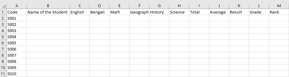
tart by preparing your column headers in Row 1 as follows:
Column Header
Ensure your headers are bold and centrally aligned for clarity.
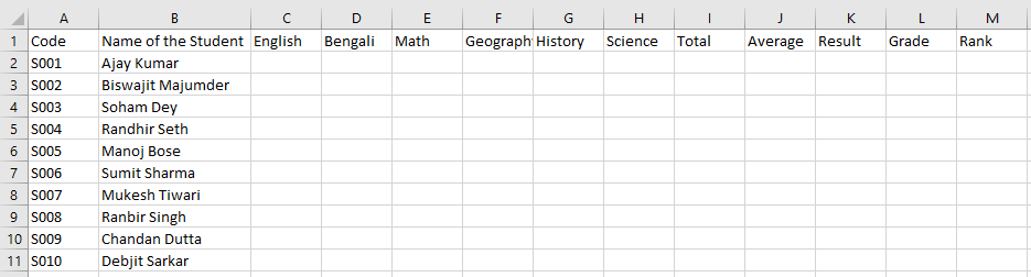
Step 2:Enter Student Information
In Column A, type:
Use a consistent format such as:
S001, S002, S003 …

In Column B, type:
Ajay Kumar, Biswajit Majumder and continue for all students.

In Columns C to G, enter subject marks for each student.
Once all marks are added, your table will start taking shape.

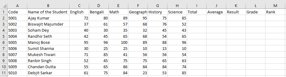
✔Ensure all marks are numeric—Excel formulas do not work with text values.
Step 3: Calculate Total Marks Using Excel Formula (SUM Function)
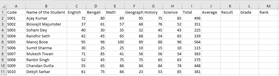
To automatically calculate a student’s total marks:
Click on I2
Enter the formula:
=SUM(C2:H2)Press Enter
This formula adds English, Bengali, Math, Geography, and History marks.
Drag the formula down to apply it to all students.
You will see the total marks for all students.

Step 4: Calculate Average / Percentage (AVERAGE Function)
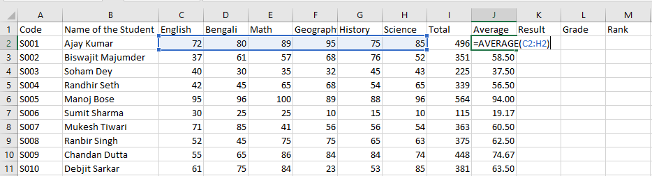
In most schools, each subject carries equal weight. In that case, the AVERAGE function is appropriate.
Click on J2
Enter the Formula =AVERAGE(C2:H2)
This calculates the percentage automatically.
Press Enter
Now drag the formula till the End.

💡 If all subjects have equal total marks, AVERAGE is correct.
Otherwise, use: Total Marks ÷ Total Maximum Marks × 100
Step 5: Determining Result – PASS or FAIL (IF Function)
Use the IF formula to determine whether the student has passed or failed.
Condition:
- Pass if Average ≥ 25
- Fail if Average < 25
In K2, type:=IF(J2>=25,”Pass”,”Fail”)
Press Enter, drag down.

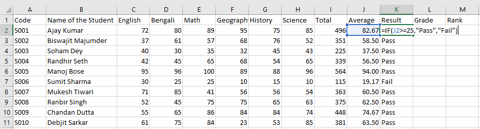
This assigns PASS or FAIL based on the calculated average.
Step 6: Grade Calculation (Nested IF Formula)
You may use the following grade distribution:
Grading Criteria
- A → 90 and above
- B → 70 and above
- C → 50 and above
- D → 35 and above
- Fail → below 35
Now we create a grading system based on the student’s average.
Formula to Calculate Grade
Click on L2 and enter:
=IF(J2>=90,"A",IF(J2>=70,"B",IF(J2>=50,"C",IF(J2>=35,"D",IF(J2>=25,"E","F")))))Hit Enter.
Copy the formula down to apply grading for all students.

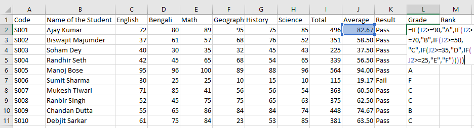
✔ Why We Use Nested IF
- A nested IF allows Excel to check multiple conditions step-by-step.
- This formula automatically assigns the correct grade according to the percentage.
Step 7: Apply the Marksheet Rank Formula in Excel (RANK Function)
This is the most crucial part of the entire marksheet.
Ranking helps identify the top-performing students in the class.
To apply the rank formula in Excel, we use the RANK function on the Total column.
In M2, type: ==RANK(I2,$I$2:$I$11,0)
Explanation:
- H2 → Student’s total marks
- $H$2:$H$11 → The entire range of total marks
- 0 → Higher marks get a better (smaller) rank

This gives an accurate, descending rank order.
Drag the formula down to assign ranks to all students.
Step 8: Professional Tips & Common Issues
A polished, trouble-free marksheet depends on a few best practices:
✔ Avoid Merged Cells
Merged cells interfere with filtering and formula application.
✔ Use Absolute References in Rank Formula
The $ symbol ensures accuracy when copying formulas.
✔ Ensure Marks Are Numeric
If marks are imported from another system, convert text to numbers using:
Data → Text to Columns → Finish
✔ Maintain Uniform Formatting
Use consistent fonts, alignments, and border styles to improve readability.
Complete List of Formulas Used
| Column | Value / Formula |
| H (Total) | =SUM(C2:H2) |
| I (Average) | =AVERAGE(C2:H2) |
| J (Result) | =IF(J2>=25,”Pass”,”Fail”) |
| K (Grade) | =IF(J2>=90,”A”,IF(J2>=70,”B”,IF(J2>=50,”C”,IF(J2>=35,”D”,IF(J2>=25,”E”,”F”))))) |
| L (Rank) | =RANK(I2,$I$2:$I$11,0)2 |
Pro Tips
Here are some extra suggestions to make your marksheet more powerful:
1.Freeze Header Rows for Easier Navigation
Go to View → Freeze Panes → Freeze Top Row.
This keeps your headings visible even when working with long student lists.
2.Protect Formula Cells to Prevent Accidental Edits
Select the formula cells → Right-click → Format Cells → Protection → Locked.
Then protect the sheet.
This prevents breaking formulas like the Excel rank function or grade logic.
3.Apply Conditional Formatting for Instant Insights
Highlight low marks, top performers, or specific subjects using icon sets or color scales. This helps track performance at a glance.
4. Add Notes or Remarks for Better Tracking
Create a small “Remarks” column to capture strengths, weaknesses, or teacher comments. This turns a simple marksheet into a performance tracker.
5. Save as a Reusable Template
Once your marksheet layout is perfect, save it as a template (.xltx) so you can reuse the structure every session without rebuilding.
Frequently Asked Questions (FAQ)
1. What is the marksheet rank formula in Excel?
The formula is:
=RANK(H2,$H$2:$H$11,0)
It assigns ranks based on Total Marks.
2. Should I use Rank based on Total or Average?
Always use Total Marks, as it reflects complete subject performance.
3. My Rank is showing duplicates. What should I do?
Duplicate marks naturally produce duplicate ranks.
See Adavnce Marksheet Tutorial
4. Why is my SUM function giving errors?
Your marks may be stored as text. Convert them to numbers.
5. Can Excel generate grades automatically?
Yes, using nested IF formulas or a VLOOKUP-based grading system.
Conclusion
A well-structured Excel marksheet is more than just a table—it is a reliable academic record and an essential tool for evaluating student performance. By using formulas like SUM, AVERAGE, IF, and the marksheet rank formula in Excel, you can build a fully automated and highly accurate grade sheet.
This professional method ensures consistency, transparency, and ease of use, both for educators and students.


